Understanding the pricing of options through binomial option pricing models

The world of finance and stock markets has a lot of complex instruments and tools used to evaluate and manage risk. One such tool is the binomial option pricing model, which provides a method for valuing options. 

Let us delve into the binomial option pricing model, breaking down its components and explaining how it works. By the end, you will have a better grasp of this concept and how it works. 

What are options?

Options are derivative financial tools that provide their owners with the option, but no compulsion, to purchase or sell an underlying asset at a pre-agreed price (referred to as the strike price) on or before a particular date.

These options come in two main categories: 

Call options: They grant the holder the privilege without any compulsion, to buy the underlying asset at the strike price on the expiry date. 

Put options: They grant the holder the privilege to sell the underlying asset at the strike price on expiry. The holder has no compulsion to fulfil the contract. 

Options are used for hedging against price fluctuations, speculating on price movements, and even generating income.

You may also like: Understanding the Black Scholes pricing model

What is the binomial option pricing model?

The fundamental approach for computing the binomial option model involves using uniform probabilities for success and failure in each period until the option reaches maturity. A trader is allowed to use different probabilities in different periods. 

Constructing the tree is straightforward, but the issue lies in the limited possible values the underlying asset can assume within a single period. In the context of a binomial tree model, the underlying asset can only possess one of two distinct values, a scenario that is not real, given that assets can potentially have numerous values within a given range.

For instance, there might exist an equal probability of a 30 per cent increase or decrease in the underlying asset’s price during a single period. However, in the next period, the likelihood of an upward movement in the underlying asset’s price could shift to 70/30.

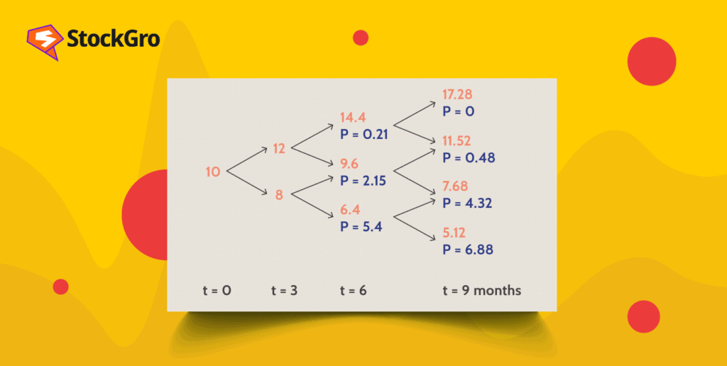
Let’s illustrate the binomial option pricing model with a simplified example. 

Binomial models for option valuation

The binomial model operates on the premise that when an asset reaches maturity, its current spot price, denoted as ‘S0’, can either rise to ‘S1u’ or fall to ‘S1d’. There is no need to possess prior knowledge about the asset’s future price, as it is contingent on the outcome of a random variable. The shifts in the asset’s price, moving from ‘S0’ to either ‘S1u’ or ‘S1d’, can be likened to the result of a Bernoulli trial (A random experiment with two possible outcomes “success” and “failure” the results of which are independent between trials)

Let us represent the probability of an uptick in the asset’s price as ‘q.’ We can denote the likelihood of a price decline as 1 – q, since there are only two possible outcomes. 

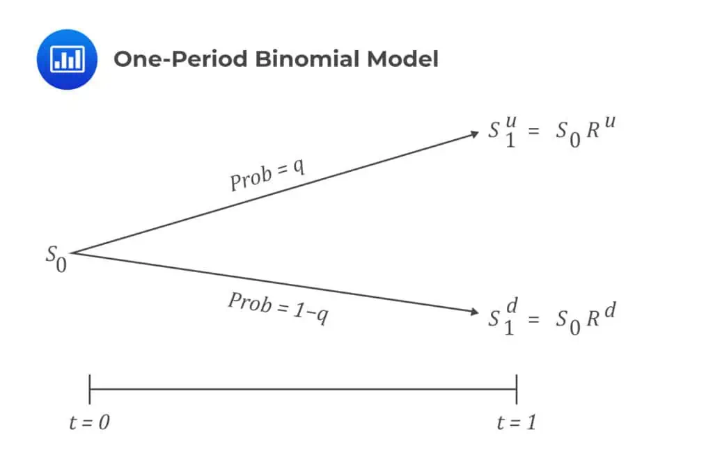
Let us contemplate a one-year call option scenario involving an initial underlying price denoted as ‘S0’ and an exercise price set at X. Additionally, let’s assume that the strike price X lies between ‘S1u’ and ‘S1d’. We are working with the one-period binomial model, which corresponds to a one-year time frame.

In this context, the one-period binomial model provides us with the future values of the underlying asset after one year, and the option’s value is determined based on these underlying values.

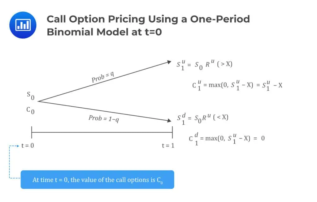
Binomial option pricing model formula:

At t=0, we do not know about Co and it needs to be computed.

At t=1, the option expires.

Value of C1u, when the price is S1u is max(0, Su-X)

Value of C1d, when the price is S1d is max(0, Sd-X). 

The value of Co is computed by the average weighing the value of C1u and C1d and pulling it back for one period by the risk-free rate.

S1u and S1d represent the upward and downward movement of the price.

“t” is the time period.

Co is the value of a call option at the zero time stamp.

C1u is the value of the call option at time period 1 when the price moves up in S1u. 

C1d is the value of the call option at time period 1 when the price moves down to S1d. 

When price rises to S1u, the call option is in the money,

For S1d, the call option is out of the money.

Also read: What is spot market?

Differences between the binomial option pricing model and the black Scholes pricing model

The Black-Scholes model suggests that an option possesses a single, correct value at the time of assessment. Conversely, the binomial model takes a dynamic approach, computing how the option’s value evolves with time. This model refrains from implying a single current value; instead, it provides a range of potential values over time.

The Black-Scholes model operates as a model where users input the required parameters, and the model yields a result. In contrast, the binomial model offers transparency, allowing users to visualise how option prices change over time. This transparency opens up various applications for the model, enabling users to input different probabilities for each period, offering a more versatile tool for option valuation.

Advantages and limitations

The Binomial Option Pricing Model has several advantages:

• It’s suitable for valuing American-style options, which can be exercised before expiration.
• The model is conceptually straightforward to understand, making it accessible to users.
• The BOPM can handle various options, including those with complex features.

However, it also has limitations:

• The model can be computationally intensive, especially when dealing with many time steps or complex option structures.
• The accuracy of the model depends on the number of time steps used, and it may require a substantial number of steps for precise results. Binomial models are used for option valuation examination and improvement convergence.

Also read: Option chain for smarter online trading

Conclusion

The BOPM is a powerful tool for calculating the value of call options. While it has its computational challenges, its ability to handle complex option structures and real-world scenarios makes it a valuable asset in the world of finance. Understanding the BOPM can empower traders and investors to make more informed decisions in the dynamic world of options trading.